Level set method

The level set method, widely used in shape optimization, consists in representing a shape $\Omega \subset D$ by a function $\phi$ which satisfies $$ \begin{cases} \phi(x) < 0 & x \in \Omega, \\ \phi(x) = 0 & x \in \partial \Omega, \\ \phi(x) > 0 & x \in D \setminus \bar{\Omega}, \\ \end{cases} $$ where $D$ is some "working domain" containing all possible shapes of interest. The main advantage of this method lies in its capacity to handle topological changes, contrary to geometric shape optimization approaches based on mesh deformation.

Usually, the level set function is discretized as a piecewise linear function on a fixed mesh of the working domain $D$. However, this comes with certains shortcomings. For instance, the level of details of the shape is fixed in advance by the mesh of $D$, and it is necessary to approximate certain geometric quantity of interest, like the mean curvature of the boundary. Moreover, the fact that the domain $\Omega$ is not explicitly meshed makes necessary the use of some ersatz material on $D \setminus \Omega$ to solve the PDE associated to the shape optimization problem, for which the formulation might not be straightforward. Finally, some geometric constraints like convexity is not straightforward to take into account with this representation of the shape.

Neural Network parametrization

One way to overcome some of the previous issues is to represent the level set function as a Neural Network $\phi_\theta$, where $\theta$ represents the parameters of the nework. This simple representation has several advantages.

Computation of local quantities

One of the main advantages of this representation is the easy and accurate computation of geometric quantities using automatic differentiation. For instance, the extended normal vector field $n_\Omega$ of $\partial \Omega$ is given by $$ n_\Omega(x) := \frac{\nabla \phi_\theta(x)}{|\nabla \phi_\theta(x)|} $$ for all $x \in D$ with $\nabla\phi_\theta(x)\neq 0$, which can be automatically computed using backpropagation. The mean curvature, which appears for instance in the shape derivative of the perimeter functional, can be computed as $$ \kappa_\Omega(x) = \text{div} n_\Omega(x) = \text{div} \left(\frac{\nabla \phi_\theta(x)}{|\nabla \phi_\theta(x)|}\right). $$

Computation of global quantities

Using a Monte Carlo approach we approximate integral quantities like the volume $\text{Vol}(\Omega)$ and the perimeter $$ \text{Per}(\Omega) := \int_{\partial \Omega} n_\Omega \cdot n_\Omega ds = \int_{\Omega} \text{div} n_\Omega d x = \int_{\Omega} \kappa_\Omega dx $$ based on i.i.d. random variables $\{x_i\}_{1\leq i \leq N}$, distributed uniformly in $D$, as $$ \text{Vol}(\Omega) \approx \frac{1}{N} \sum_{i=1}^N 1_{\{\phi_\theta < 0\}}(x_i) \quad \mbox{and} \quad \text{Per}(\Omega) \approx \frac{1}{N} \sum_{i=1}^N 1_{\{\phi_\theta < 0\}}(x_i) \kappa_\Omega(x_i). $$

Since Monte-Carlo doesn't suffer from the curse of dimensionality, this approach could be useful in high-dimensional shape optimization.

Convexity constraint

Theoretical shape optimization often deals with optimization in the class of convex sets. Being able to perform convex shape optimization numerically allows to provide powerful experimental conjectures. In our framework, we can "force" the convexity constraint in the architecture of the network: for $\sigma : \mathbb{R} \to \mathbb{R}$ we consider the following 1-layer neural network: \begin{equation} \label{eq:convex_ls} \phi_\theta(x) := W_2 \sigma(W_1x+b_1) + b_2. \end{equation} If $\sigma$ is convex and all entries of $W_2$ are non-negative, then $\phi_\theta : \mathbb{R}^d \to \mathbb{R}$ is a convex function and the shape $\Omega := \{\phi_\theta < 0\}$ is convex.

Numerical results

Using the previously described approach, we are interested in the shape optimization problem $$ \max_{\text{Vol}(\Omega)=1} \mu_k(\Omega) $$ where $\mu_k(\Omega)$ is the $k$-th eigenvalue of the Neumann eigenvalue problem $$ \begin{cases} -\Delta u = \mu_k(\Omega) u &\mbox { in } \Omega,\\ \frac{\partial u}{\partial n} = 0 &\mbox { on } \partial \Omega. \end{cases} $$ The choice of this particular problem is motivated by the graph-based PDE solver that we used, for which the previous problem is the natural continuous counterpart. More details can be found here and in the companion article.

2D results

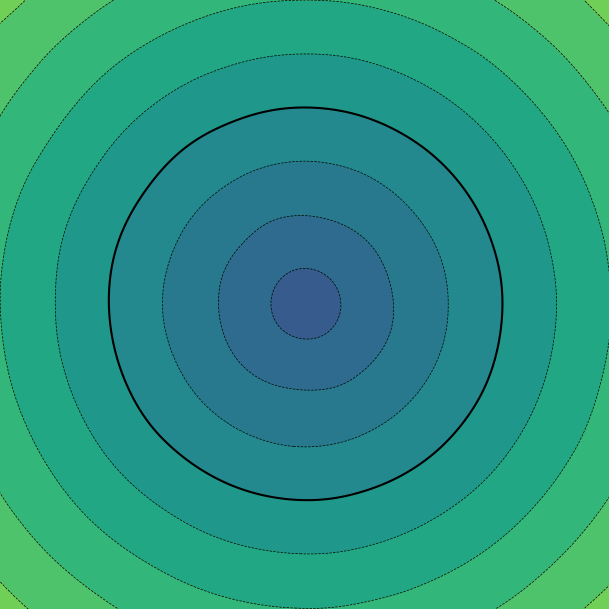
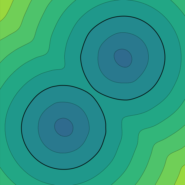
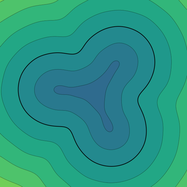
We present the results of the method in 2D. We plot the level set function $\phi_\theta$, where the thick black line represents the $0$ level set (the shape). From left to right, we have: the initial level set, and the optimized shapes for $\mu_1, \mu_2$ and $\mu_3$.

3D results

We represent the convergence of the method for the optimization of $\mu_1, \mu_2$ and $\mu_3$. Only the $0$ level set is plotted.

This project was a lot of fun and brought a lot of simple yet nice ideas. I think there is still plenty that can be done using neural networks for the representation of shapes. More information can be found in the companion article.