Presentation of the problem

The level set approach is complementary to the density one. In this framework however we stick with the original shape optimization problem. Let's recall the main lines : Let $\mathbb{S}^N \in \mathbb{R}^{N+1}$, $N \geq 1$ be the unit sphere and $\Omega \subset \mathbb{S}^N$ be an open set with Lipschitz boundary. By the spectral theorem, there exists a sequence $$ 0 = \mu_0(\Omega) \leq \mu_1(\Omega) \leq ... \to \infty $$ such that $$ \begin{cases} -\Delta u = \mu_k(\Omega) u \mbox { in } \Omega,\\ \frac{\partial u}{\partial n} = 0 \mbox { on } \partial \Omega, \end{cases} $$ for some $u \in H^1(\Omega) \setminus \{0\}$. Here, $\Delta$ denotes the Laplace-Beltrami operator (the generalization of the Lapalce operator on curved spaces). The $\mu_k(\Omega)$ are called the eigenvalues of the Laplace operator with Neumann boundary conditions and the associated $u$ is called an eigenfunction. For a given $k \in \mathbb{N}$ and a given volume $m > 0$, the problem is to find the domain $\Omega$ which maximizes the eigenvalue $\mu_k(\Omega)$ with $|\Omega| = m$ $$ \max \left\{ \mu_k(\Omega) : \Omega \subset \mathbb{R}^N, |\Omega| =m\right\}. $$ The well knows Courant-Hilbert formula allows us to express the eigenvalues in the following manner : $$ \mu_k(\Omega) = \min_{S\in{\mathcal S}_{k+1}} \max_{u \in S\setminus \{0\}} \frac{\int_\Omega |\nabla u|^2 dx}{\int_\Omega u^2 dx}, $$ where ${\mathcal S}_k$ is the family of all subspaces of dimension $k$ in $H^1(\Omega)$.

Principle of the level set method

One concern in numerical shape optimization is to determine a good parametrization of the shape $\Omega$. The first idea that may come up is to represent it by a mesh. However, numerical optimization algorithm will make the shape move and this parametrization might be inadapted if we want to handle some topological changes.

One way to handle this is throug the level set method. Instead of describing the evolving shape as a moving mesh, we describe it as an evolving function on a fixed mesh. More precisely, if we have a continuous family of shapes $\left(\Omega_t\right)_t$ then it will be represented as the zero sub-level set of a function $\phi$ : $$ \forall x \in \mathbb{S}^N, \forall t\in[0,T], \begin{cases} \phi(t,x) < 0 & \mbox{ if } x \in \Omega_t \\ \phi(t, x) = 0 & \mbox{ if } x \in \partial \Omega_t \\ \phi(t,x) > 0 & \mbox{ if } x \in \mathbb{S}^N \setminus \Omega_t \end{cases}. $$ Let's now suppose that the family $\Omega_t$ is advected by a velocity field $V : \mathbb{R}^+\times \mathbb{S}^N \to T \mathbb{S}^N$ in such a way that $\Omega_t = \chi(\Omega_0,t)$ where $$ \begin{cases} \chi'(x_0,t)= V(t,\chi(x_0,t)) \mbox{ for } (t,x_0) \in \mathbb{R}^+\times \mathbb{S}^N \\ \chi(x_0,0)= x_0 \in \mathbb{S}^N \end{cases} $$ The advantage of this representation is that the motion of $\Omega_t$ is equivalent to the advection of $\phi$ by the equation $$ \partial_t \phi(t,x) + V(t,x) \cdot \nabla \phi(t,x) = 0. $$ During a single time step $t_m \to t_{m+1}$, we can consider $V(t,x) \approx V_m(x)$ and solve $$ \partial_t \phi(t,x) + V_m(x) \cdot \nabla \phi(t,x) = 0 $$ instead. At each time step, this equation can be solved using, for instance, the method of characteristics.

Knowing how to paramterize the shape, we should know find at each time step $t_m$ a velocity field $V_m$ which makes the eigenvalue $\mu_k(\Omega_{t_m})$ increase. This is done using the concept of shape derivative, which will be covered in another post.

You can learn more about the shape optimization using the level set method by checking the amazing web page of Charles Dapogny which has a lot of wonderful resources. You can also check [1].

Numerical explorations for the first three eigenvalues

We use a gradient-based optimization algorithm with a penalization of the surface to take the constraint into account. For more information, we refer to the companion article.

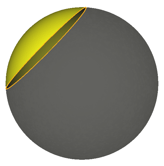
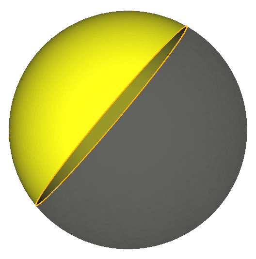
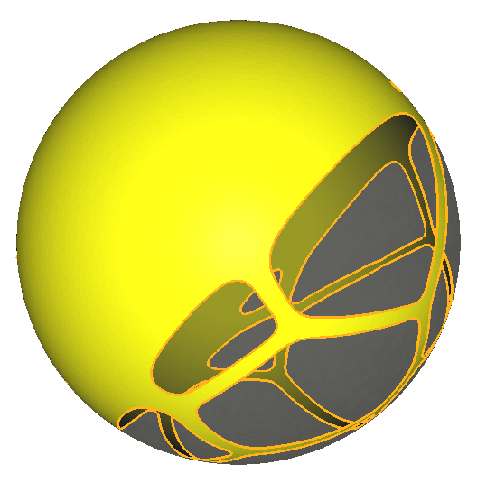
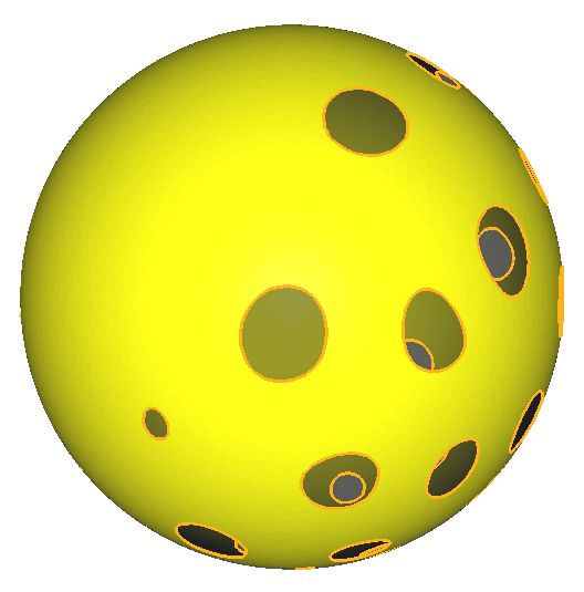
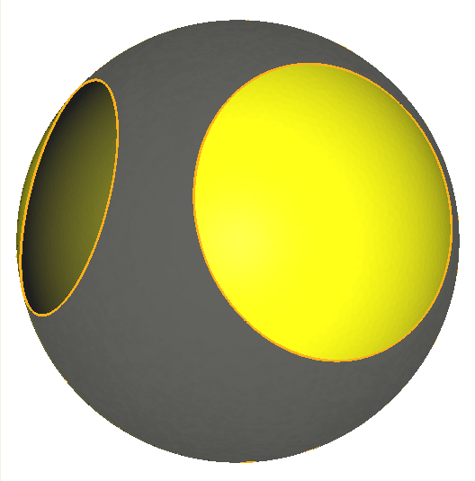
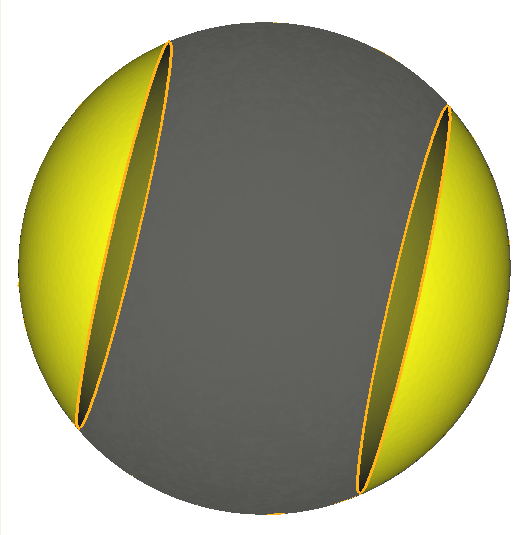
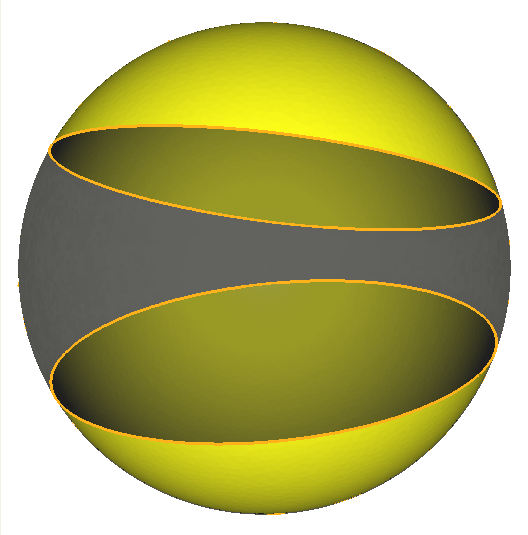
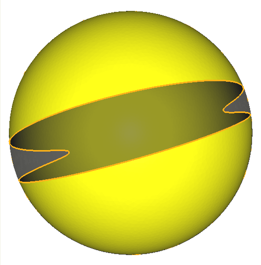
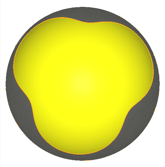
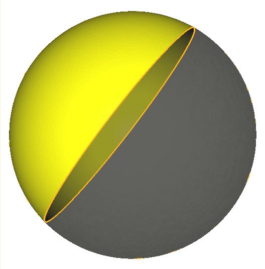
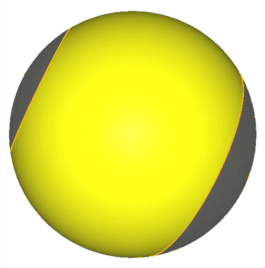
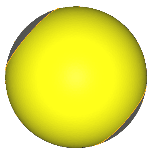
The pictures above represents the optimal shapes for $\mu_1, \mu_2$ and $\mu_3$ (first, second and third row) obtained for $m \in \{2, 5, 8, 11\}$ (in column). The most important observation we can make is the following :

This observation goes in contrast to the theorem of Laugesen and Langford [2] where under the hypothesis of simple conectedness, the geodesic ball is proven to be optimal for $0 < M < 0.94 |\mathbb{S}^N$. It shows that this topological assumption can't be dropped.

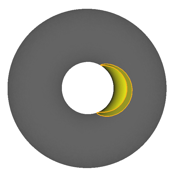
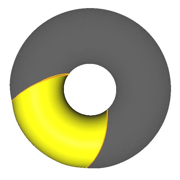
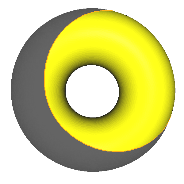
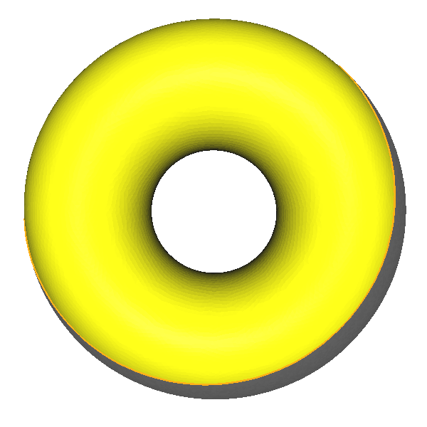
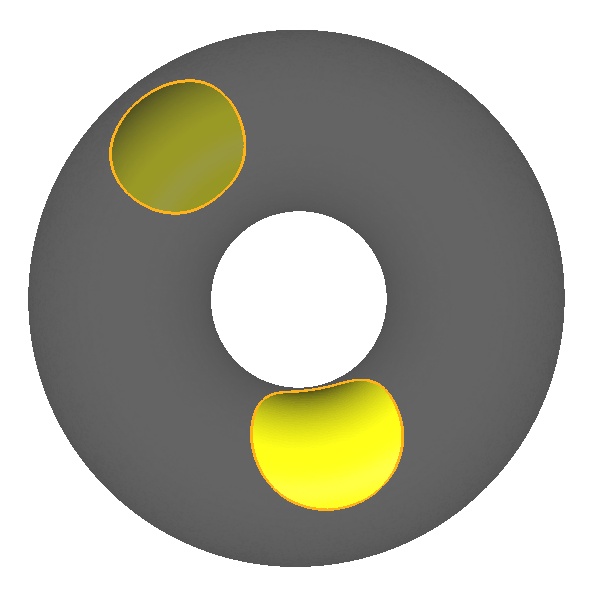
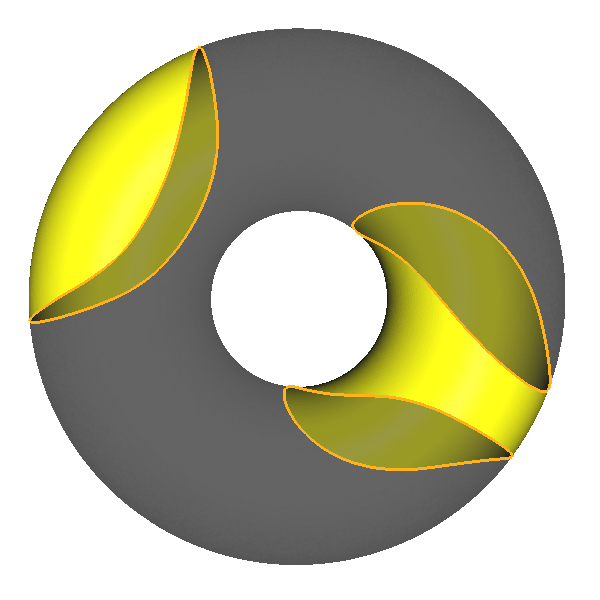
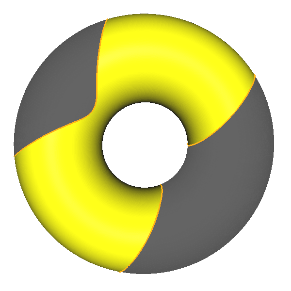
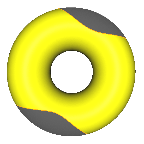
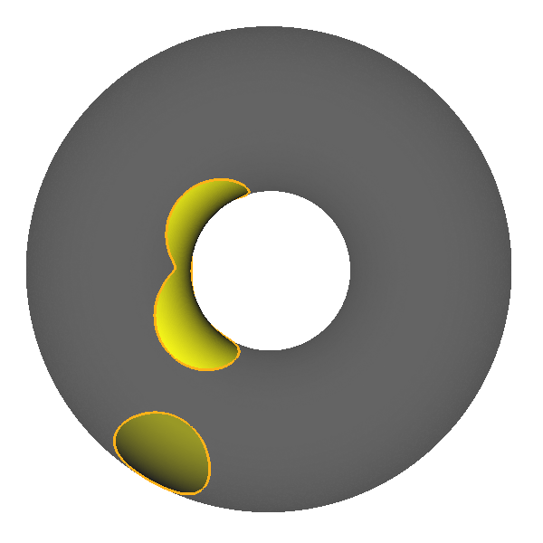
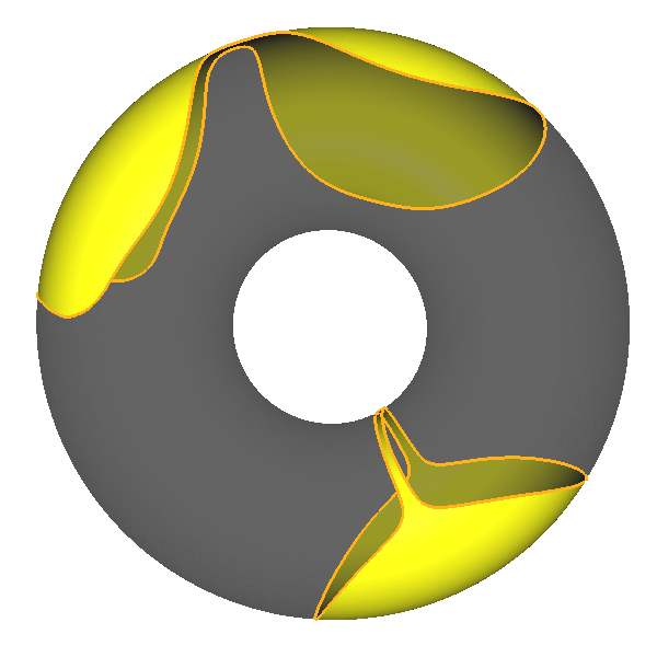
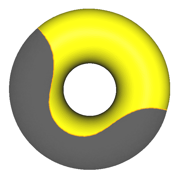
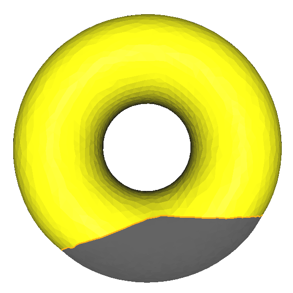
Same simulations on the torus

Only for the pleasure of the eyes, here are the same simulations on the torus :

Once again, I encourage you to check the associated paper and to send me an email if you need more informations !