Presentation of the problem

The framework is largely the same as the one presented here but we recall the main ideas. Let $\mathbb{S}^N \in \mathbb{R}^{N+1}$, $N \geq 1$ be the unit sphere and $\Omega \subset \mathbb{S}^N$ be an open set with Lipschitz boundary. By the spectral theorem, there exists a sequence $$ 0 = \mu_0(\Omega) \leq \mu_1(\Omega) \leq ... \to \infty $$ such that $$ \begin{cases} -\Delta u = \mu_k(\Omega) u \mbox { in } \Omega,\\ \frac{\partial u}{\partial n} = 0 \mbox { on } \partial \Omega, \end{cases} $$ for some $u \in H^1(\Omega) \setminus \{0\}$. Here, $\Delta$ denotes the Laplace-Beltrami operator (the generalization of the Lapalce operator on curved spaces). The $\mu_k(\Omega)$ are called the eigenvalues of the Laplace operator with Neumann boundary conditions and the associated $u$ is called an eigenfunction. For a given $k \in \mathbb{N}$ and a given volume $m > 0$, the problem is to find the domain $\Omega$ which maximizes the eigenvalue $\mu_k(\Omega)$ with $|\Omega| = m$ $$ \max \left\{ \mu_k(\Omega) : \Omega \subset \mathbb{R}^N, |\Omega| =m\right\}. $$ The well knows Courant-Hilbert formula allows us to express the eigenvalues in the following manner : $$ \mu_k(\Omega) = \min_{S\in{\mathcal S}_{k+1}} \max_{u \in S\setminus \{0\}} \frac{\int_\Omega |\nabla u|^2 dx}{\int_\Omega u^2 dx}, $$ where ${\mathcal S}_k$ is the family of all subspaces of dimension $k$ in $H^1(\Omega)$.

Extension to densities

Until recently, no one known what the solution were for this problem, for any $N$, $m$ and $k$ in full generality. However, some properties have been deduced from strong assumptions on $\Omega$, see for instance [1] or [2]. In the line of the planar optimization, we extend our definition of eigenvalues in a class of densitites. Let $\rho : \mathbb{S}^N \to [0,1]$ such that $0<\int_{\mathbb{S}^N} \rho dx < |\mathbb{S}^N|$. We define $$ \mu _k(\rho) := \inf_{S\in{\mathcal S}_{k+1}} \max_{u \in S} \frac{\int_{\mathbb{S}^N} \rho|\nabla u|^2 dx}{\int_{\mathbb{S}^N} \rho u^2 dx}, $$ where ${\mathcal S}_{k+1}$ is the family of all subspaces of dimension $k+1$ in $$ \{u\cdot 1_{\{\rho (x)>0\}}: u \in C^\infty_c (\mathbb{S}^N)\}. $$ and $\nabla$ is the tangential gradient. Our maximization problem becomes : $$ \begin{equation} \label{bmo01} \sup \left\{ \mu_k(\rho) : \rho : \mathbb{R}^N \to [0,1], \int_{\mathbb{R}^N}\rho dx =m\right\}. \end{equation} $$

Numerical explorations: results for $\mu_1$

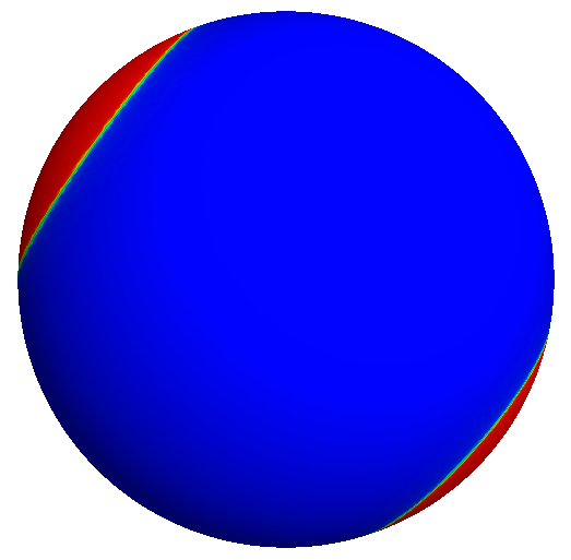
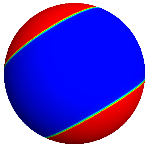
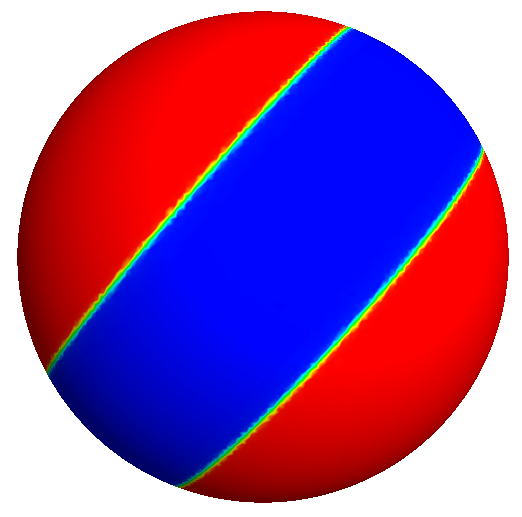
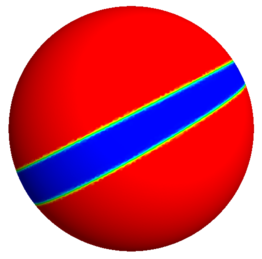
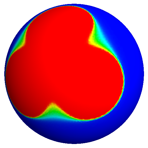
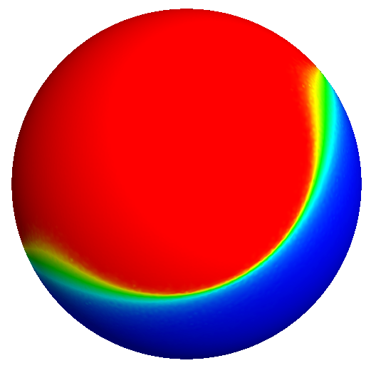
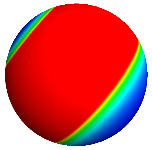
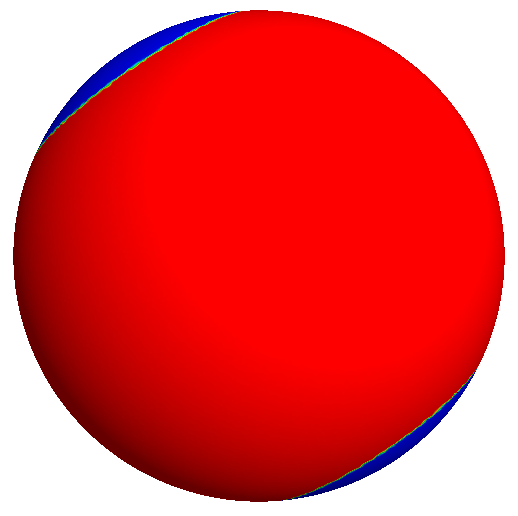
The optimization procedure is the same as in the planar case. One of the main question was to know whether the geodesic disk was still optimal for $\mu_1$ in the density framework without any assumption. It turned out it wasn't the case :

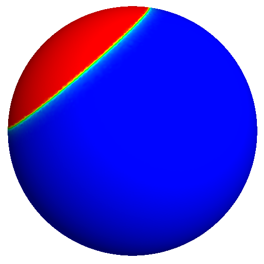
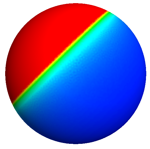
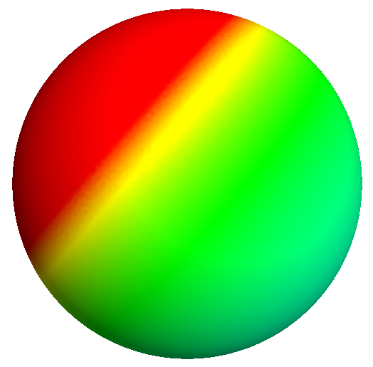
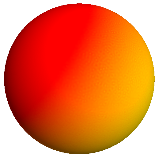
The pictures above represents the optimal densites obtained for $m \in \{2, 5, 8, 11\}$ (approx). The red color represents $\rho=1$ while the blue one represents $\rho=0$. Here, we clearly see that for enough mass, we can find a better density than the one of the geodesic cap.

Numerical explorations: results for $\mu_2$

Contrary to $\mu_1$ for which the numerical experiments only highlighted the strange (and interesting !) behaviour, the case of $\mu_2$ is pretty clear :

Once again, we represent the optimal densities for a wide range of values of $m$. We directly observe that the optimal densities are always the characteristic function of two disjoint geodesic caps. This is, indeed, a fact :

The demonstration can be found in the companion article Sharp inequalities for Neumann eigenvalues on the sphere written with Dorin Bucur and Mickaël Nahon.

Numerical explorations: results for $\mu_3$

We already saw interesting things for the two first eigenvalues on the sphere, so, why not iterate the process ? Here are some results for $\mu_3$, with $m \in \{2,5,8,11\}$:

I don't want to do more comments here, appart that I hope you enjoy as much as I do the aesthetic beauty of these pictures. If you want to know more about the simulations, I encourage you to check the companion article. Don't hesistate to contact me either, I would be glad to answer your questions !

Bonus

Those computations may actually be performed for any 2 dimensional surface. For instance, here is the optimization process for $\mu_3$ on a coarse mesh of a torus :